OpenCV高级操作

阈值处理

阈值处理有很多种，有三种形式：

手动提供参数来设定合适的阈值分割图像。需要控制照明条件下工作得非常好，可以确保图像的前景和背景之间的高对比度。
如OTSU阈值之类的方法，这些方法试图更动态地自动计算最佳阈值。
自适应阈值，它不是试图用一个单一的值全局地阈值一个图像，而是把图像分解成更小的部分，然后分别地和单独地对每个部分进行阈值。

手动阈值 Basic thresholding

需要手动确定阈值T

# apply basic thresholding -- the first parameter is the image
# we want to threshold, the second value is is our threshold
# check; if a pixel value is greater than our threshold (in this
# case, 200), we set it to be *black, otherwise it is *white*
(T, threshInv) = cv2.threshold(blurred, 200, 255,
	cv2.THRESH_BINARY_INV)
cv2.imshow("Threshold Binary Inverse", threshInv)

cv2.threshold 第一个参数为需要处理的图像，第二个为阈值T，第三个为高于阈值后需要变化为的数值（通常为255，表示变为黑色），第四个为阈值处理方法。
输出结果第一个T表示阈值，第二个表示阈值后的图像。

自动化阈值 OTSU

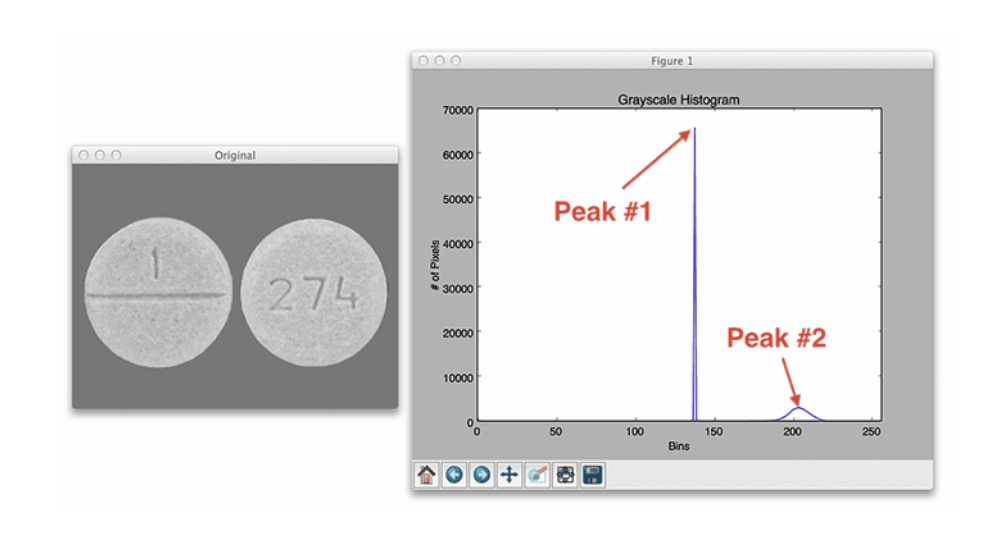
OTUS可以帮助我们自动设置阈值。Otsu的方法假设我们的图像像素强度的灰度直方图是双模态的，这仅仅意味着直方图是两个峰。[[opencv直方图对比|直方图详解]]

例如如下图像，第一个尖峰对应于图像的统一背景颜色，而第二个峰值对应于药丸区域本身。

(T, threshInv) = cv2.threshold(blurred, 0, 255,
	cv2.THRESH_BINARY_INV | cv2.THRESH_OTSU)

使用OTSU第二个参数设置为了0，因为它会自动帮助我们计算阈值。

import argparse  
import cv2  
ap = argparse.ArgumentParser()  
ap.add_argument("-i", "--image", type=str, required=True,  
   help="path to input image")  
args = vars(ap.parse_args())  
  
# load the image and display it  
image = cv2.imread(args["image"])  
cv2.imshow("Image", image)  
# convert the image to grayscale and blur it slightly  
gray = cv2.cvtColor(image, cv2.COLOR_BGR2GRAY)  
blurred = cv2.GaussianBlur(gray, (7, 7), 0)  
  
# apply Otsu's automatic thresholding which automatically determines  
# the best threshold value  
(T, threshInv) = cv2.threshold(blurred, 0, 255,  
   cv2.THRESH_BINARY_INV | cv2.THRESH_OTSU)  
cv2.imshow("Threshold", threshInv)  
print("[INFO] otsu's thresholding value: {}".format(T))  
# visualize only the masked regions in the image  
masked = cv2.bitwise_and(image, image, mask=threshInv)  
cv2.imshow("Output", masked)  
cv2.waitKey(0)

注意一下cv2.threshold 中的阈值方法参数：

cv2.THRESH_BINARY_INV 二值化后再反转
cv2.THRESH_BINARY 正常二值化

参考 OpenCV Thresholding ( cv2.threshold ) - PyImageSearch

自适应阈值 adaptive thresholding

对于一些复杂的图像，全局只有一个阈值分割效果可能会不好，因此使用自适应阈值。而且可以避免训练专用Mask R-CNN或U-Net分割网络的耗时和计算昂贵的过程。

具体思想是在小块的领域确定阈值，选取区域大小是个需要调整的参数。区域阈值计算方法可以选择算术平均值或高斯平均值，算数平均更加常用。

thresh = cv2.adaptiveThreshold(blurred, 255,
	cv2.ADAPTIVE_THRESH_MEAN_C, cv2.THRESH_BINARY_INV, 21, 10)

输入参数第一个为目标图像；第二个为输入阈值；第三个为自适应阈值方法，可选cv2.ADAPTIVE_THRESH_MEAN_C 或 cv2.ADAPTIVE_THRESH_GAUSSIAN_C ；第四个如同手动阈值方法；第五个是领域大小，这里表示21×21；最后一个为微调常数值C，通过加减C来进行调整阈值。

image = cv2.imread('test.png')
cv2.imshow("Image", image)
# convert the image to grayscale and blur it slightly
gray = cv2.cvtColor(image, cv2.COLOR_BGR2GRAY)
blurred = cv2.GaussianBlur(gray, (7, 7), 0)

# instead of manually specifying the threshold value, we can use
# adaptive thresholding to examine neighborhoods of pixels and
# adaptively threshold each neighborhood
thresh = cv2.adaptiveThreshold(blurred, 255,
	cv2.ADAPTIVE_THRESH_MEAN_C, cv2.THRESH_BINARY_INV, 21, 4)
cv2.imshow("Mean Adaptive Thresholding", thresh)
cv2.waitKey(0)

参考 Adaptive Thresholding with OpenCV ( cv2.adaptiveThreshold )

图像平滑和模糊

平滑和模糊是计算机视觉和图像处理中最常见的预处理步骤之一。在应用边缘检测或阈值分割等技术之前，通过平滑图像，能够减少高频内容的数量，如噪声和边缘(即图像的细节)。

平均模糊 cv2.blur

取中心像素周围的像素区域，将所有这些像素平均在一起，并用平均值替换中心像素。通常使用 M×N (M N为奇数)的内核进行平均。随着内核大小的增加，图像模糊的数量也会增加。

kernelSizes = [(3, 3), (9, 9), (15, 15)]
# loop over the kernel sizes
for (kX, kY) in kernelSizes:
	# apply an "average" blur to the image using the current kernel
	# size
	blurred = cv2.blur(image, (kX, kY))
	cv2.imshow("Average ({}, {})".format(kX, kY), blurred)
	cv2.waitKey(0)

高斯模糊 cv2.GaussianBlur

高斯模糊类似于平均模糊，但不是简单的平均值，而是加权平均值，其中更接近中心像素的邻域像素对平均值贡献更多的权重。借助M×N 的内核(M N为奇数)，基于这种加权，将能够保留图像中更多的边缘。

x和y方向上的高斯函数如下：

G(x,y)= \frac{1}{2 \pi \sigma}e^{- \frac{x^{2}+y^{2}}{2 \sigma ^{2}}}

当内核的大小增加时，应用于输出图像的模糊量也会增加。

kernelSizes = [(3, 3), (9, 9), (15, 15)]
# loop over the kernel sizes again
for (kX, kY) in kernelSizes:
	# apply a "Gaussian" blur to the image
	blurred = cv2.GaussianBlur(image, (kX, kY), 0)
	cv2.imshow("Gaussian ({}, {})".format(kX, kY), blurred)
	cv2.waitKey(0)

最后一个参数为高斯分布的标准差。通过将这个值设置为0，我们指示OpenCV根据内核大小自动计算。更多细节可以参考 OpenCV documentation

中值模糊 cv2.medianBlur

中值模糊方法是去除椒盐噪声最有效的方法。该方法的内核大小必须是正方形。并且用邻域的中值代替中心像素。

中值模糊在从图像中去除椒盐风格噪声时更有效的原因是每个中心像素总是被图像中存在的像素强度所取代。由于中位数对异常值具有稳健性，与平均值等其他统计方法相比，椒盐噪声对中位数的影响较小。

kernelSizes = [(3, 3), (9, 9), (15, 15)]
# loop over the kernel sizes a final time
for k in (3, 9, 15):
	# apply a "median" blur to the image
	blurred = cv2.medianBlur(image, k)
	cv2.imshow("Median {}".format(k), blurred)
	cv2.waitKey(0)

双边模糊 cv2.bilateralFilter

上面几种模糊方法往往会失去图像的边缘，为了在保持边缘的同时减少噪声，可以使用双边模糊（利用两个高斯分布）。但是它的速度会慢很多。

blurred = cv2.bilateralFilter(image, diameter, sigmaColor, sigmaSpace)

第一个参数为需要模糊的图像；第二个参数为像素邻域的直径。直径越大，模糊计算中包含的像素就越多；第三个参数是颜色标准偏差，更大的值意味着在计算模糊时将考虑附近更多的颜色。第四个参数为坐标空间中的sigma值。它的值越大，说明有越多的点能够参与到滤波计算中来。

参考 OpenCV Smoothing and Blurring - PyImageSearch

形态学操作

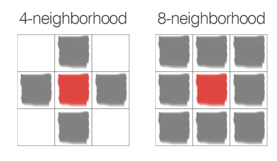
形态学运算是应用于二值或灰度图像的简单变换。形态学操作探测带有结构元素(structuring elements)的图像。这个结构元素定义了每个像素周围要检查的邻域。根据给定的操作和结构元素的大小，我们可以调整输出图像。

有时候很多东西根本不配用上特别高级的算法，例如机器学习，深度学习。

结构元素在opencv中用cv2.getStructuringElement定义，如下与定义4邻域和8邻域的一个例子

侵蚀 Erosion

图像中物体边界附近的像素将被丢弃侵蚀掉。

侵蚀通过定义结构元素，然后在输入图像上从左到右、从上到下滑动这个结构元素。只有当结构元素中的所有像素都是> 0时，输入图像中的前景像素才会被保留。否则，像素被设置为0(即背景)。

使用 cv2.erode

# apply a series of erosions
for i in range(0, 3):
	eroded = cv2.erode(gray, None, iterations=i + 1)
	cv2.imshow("Eroded {} times".format(i + 1), eroded)
	cv2.waitKey(0)

第一个参数为需要侵蚀的图像；第二个为侵蚀的结构元素，设为None表示3×3的8领域结构；第三个为膨胀迭代次数。

膨胀 dilation

膨胀可以增加前景对象的大小，尤其适用于将图像的破碎部分连接在一起。通过定义结构元素，若任意一个像素为> 0，则结构元素的中心像素p将被设置为白色。

使用 cv2.dilate

# apply a series of dilations
for i in range(0, 3):
	dilated = cv2.dilate(gray.copy(), None, iterations=i + 1)
	cv2.imshow("Dilated {} times".format(i + 1), dilated)
	cv2.waitKey(0)

参数类似侵蚀，基本同理

开操作 Opening

开操作是侵蚀之后的膨胀。该操作可以从图像中删除小斑点:首先应用侵蚀来删除小斑点，然后应用膨胀来重新增长原始对象的大小。

kernelSizes = [(3, 3), (5, 5), (7, 7)]
# loop over the kernels sizes
for kernelSize in kernelSizes:
	# construct a rectangular kernel from the current size and then
	# apply an "opening" operation
	kernel = cv2.getStructuringElement(cv2.MORPH_RECT, kernelSize)
	opening = cv2.morphologyEx(gray, cv2.MORPH_OPEN, kernel)
	cv2.imshow("Opening: ({}, {})".format(
		kernelSize[0], kernelSize[1]), opening)
	cv2.waitKey(0)

cv2.getStructuringElement用来定义一个结构元素。第一个参数结构元素类型：cv2.MORPH_RECT 表示正方形结构（8邻域），cv2.MORPH_CROSS 表示十字形结构（4邻域），cv2.MORPH_ELLIPSE 表示圆形结构。第二个参数表示大小。

这里开操作使用 cv2.morphologyEx 函数，不过实际上它能够传递任何想要的形态操作。这里操作方式选择cv2.MORPH_OPEN 表示开操作。

闭操作 Closing

闭操作是膨胀之后的侵蚀。它可以将物体内部的孔或将组件连接在一起。

kernelSizes = [(3, 3), (5, 5), (7, 7)]
for kernelSize in kernelSizes:
	# construct a rectangular kernel form the current size, but this
	# time apply a "closing" operation
	kernel = cv2.getStructuringElement(cv2.MORPH_RECT, kernelSize)
	closing = cv2.morphologyEx(gray, cv2.MORPH_CLOSE, kernel)
	cv2.imshow("Closing: ({}, {})".format(
		kernelSize[0], kernelSize[1]), closing)
	cv2.waitKey(0)

与开操作类似，不过cv2.morphologyEx 函数中方法选择 cv2.MORPH_CLOSE

形态学梯度 Morphological gradient

形态学梯度是膨胀和侵蚀之间的差异。它对于确定图像的特定对象的轮廓很有用

kernelSizes = [(3, 3), (5, 5), (7, 7)]
for kernelSize in kernelSizes:
	# construct a rectangular kernel and apply a "morphological
	# gradient" operation to the image
	kernel = cv2.getStructuringElement(cv2.MORPH_RECT, kernelSize)
	gradient = cv2.morphologyEx(gray, cv2.MORPH_GRADIENT, kernel)
	cv2.imshow("Gradient: ({}, {})".format(
		kernelSize[0], kernelSize[1]), gradient)
	cv2.waitKey(0)

cv2.morphologyEx 函数中方法选择 cv2.MORPH_GRADIENT

顶帽操作（Top hat/white hat）和黑帽操作（black hat）

top hat用于在深色背景上显示图像的明亮区域。

image = cv2.imread(args["image"])
gray = cv2.cvtColor(image, cv2.COLOR_BGR2GRAY)

# construct a rectangular kernel (13x5) and apply a blackhat
# operation which enables us to find dark regions on a light
# background
rectKernel = cv2.getStructuringElement(cv2.MORPH_RECT, (13, 5))
blackhat = cv2.morphologyEx(gray, cv2.MORPH_BLACKHAT, rectKernel)

# similarly, a tophat (also called a "whitehat") operation will
# enable us to find light regions on a dark background
tophat = cv2.morphologyEx(gray, cv2.MORPH_TOPHAT, rectKernel)

# show the output images
cv2.imshow("Original", image)
cv2.imshow("Blackhat", blackhat)
cv2.imshow("Tophat", tophat)
cv2.waitKey(0)

分别使用 cv2.MORPH_BLACKHAT 和 cv2.MORPH_TOPHAT 去进行操作

参考 OpenCV Morphological Operations

颜色空间

主要基于 cv2.cvtColor 函数

照明条件的重要性

照明条件对于计算机视觉处理流程有着重要的影响。光的质量是图像进入算法前就应该积极考虑的，它可能是最重要的因素。

高对比度 High contrast
尽量确保环境的背景和前景之间有很高的对比度，这将使编写代码更容易准确地理解背景和前景。
可推广的 Generalizable
照明条件应该足够一致，以至于它们从一个物体到另一个对象都可以很好地工作。
稳健性 Stable
拥有稳定、一致和可重复的照明条件是计算机视觉应用开发重要因素。

RGB color space

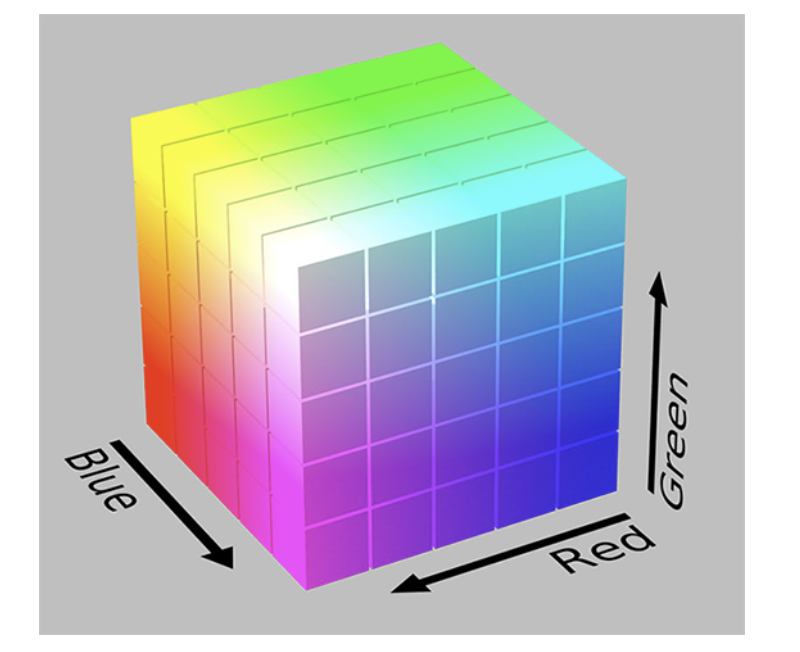
由RGB三个通道组成，每个通道范围为[0,255]。RGB颜色空间是加色空间的一个例子:每种颜色加的越多，像素就变得越亮，越接近白色。需要将三个通道都加起来才能表示一种颜色。

HSV color space

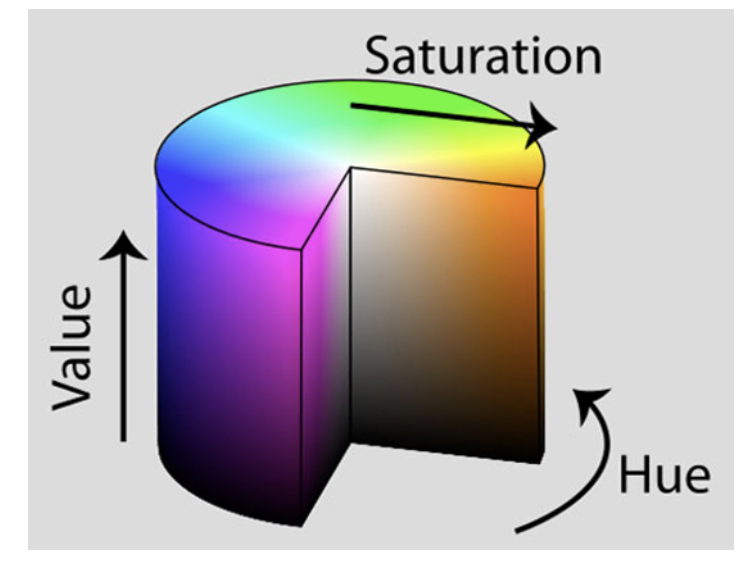
HSV颜色空间会改变RGB的颜色空间，将其重塑为圆柱体而不是立方体。在RGB部分中看到的，颜色的白色或明度是每个红色、绿色和蓝色组件的相加组合。但现在在HSV颜色空间中，亮度被赋予了自己的独立维度。

Hue：检查哪种“纯”颜色。例如，颜色“红色”的所有阴影和色调都具有相同的色调。
Saturation：颜色是多么“白色”。完全饱和的颜色将是“纯”，如“纯红色”。零饱和的颜色将是纯白色。
value：控制颜色的明度。0将表示纯黑色，而增加将产生较浅的颜色

不同的计算机视觉库将使用不同的范围来表示每个色相、饱和度和值组件。
在OpenCV中，图像表示为8位无符号整数数组。因此，Hue值被定义为范围[0,179] (总共有180个可能的值，因为[0,359]共360对于8位无符号数组是不可能的)，Hue实际上是HSV颜色圆柱上的度数。Saturation和value范围都在[0,255]。

转换方式使用cv2.COLOR_BGR2HSV

hsv = cv2.cvtColor(image, cv2.COLOR_BGR2HSV)

Value组件本质上是一个灰度图像，这是因为Value控制了颜色的实际明度，而Hue和Saturation定义了实际的颜色和阴影。HSV颜色空间在计算机视觉应用中被大量使用，特别是当我们对跟踪图像中某些物体的颜色感兴趣时。使用HSV定义一个有效的颜色范围比使用RGB要容易得多。

L* a* b* color space

该方法目标是模仿人类观察和解释颜色的方法。L* a* b* 颜色空间中任意两种颜色之间的欧几里得距离具有实际的感知意义。L* a* b* 颜色空间是一个3轴系统

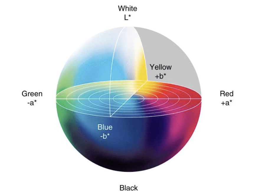
L-channel: 像素的亮度。这个值在垂直轴上上下变化，从白色到黑色，轴的中心是中性灰色。
a-channel: 源于L通道的中心，在光谱的一端定义纯绿色，在另一端定义纯红色。
b-channel：源于l通道的中心，但垂直于a通道。b通道在一个光谱上定义纯蓝色，在另一个光谱上定义纯黄色。

L* a* b* 颜色空间不像HSV和RGB颜色空间那么直观，但它在计算机视觉中被大量使用。这是因为颜色之间的距离具有实际的感知意义，使我们能够克服各种光照条件问题。它还可以作为一个强大的彩色图像描述符。

转换方式使用cv2.COLOR_BGR2LAB

lab = cv2.cvtColor(image, cv2.COLOR_BGR2LAB)

L* 通道，用于显示给定像素的亮度。然后，a* 和b* 决定像素的阴影和颜色。

灰度 Grayscale

转换方式使用cv2.COLOR_BGR2GRAY

gray = cv2.cvtColor(image, cv2.COLOR_BGR2GRAY)

转化为单一通道像素范围在[0,255]的图像。转化公式如下

Y=0.299 \times R+0.587 \times G+0.114 \times B

不平均主要是由于我们视觉感知RGB三种颜色敏感度不同。

参考 OpenCV Color Spaces ( cv2.cvtColor )

图像梯度

图像梯度的作用

使用梯度检测图像中的边缘，在图像中找到对象的轮廓，阴影，边缘等等
用作通过特征提取来量化图像的输入。例如定向梯度直方图（Histogram of Oriented Gradients）和 SIFT
用于构建显着图（saliency maps），突出显示图像的主题

通常检测到图像的边缘叫做edge map

关于图像梯度手动计算的方法参考这里

Sobel and Scharr kernels

Sobel使用了两个核，一个用于检测水平方向的变化，另一个用于检测垂直方向的变化

G _ { x } = \left[ \begin{array} { l l l } { - 1 } & { 0 } & { + 1 } \\ { - 2 } & { 0 } & { + 2 } \\ { - 1 } & { 0 } & { + 1 } \end{array} \right]\ and\ G _ { y } = \left[ \begin{array} { l l l } { - 1 } & { - 2 } & { - 1 } \\ { 0 } & { 0 } & { 0 } \\ { + 1 } & { + 2 } & { + 1 } \end{array} \right]

Scharr类似，不过核不太一样，效果会更好一些。

G _ { x } = \left[ \begin{array} { l l l } { - 3 } & { 0 } & { + 3 } \\ { - 10 } & { 0 } & { + 10 } \\ { - 3 } & { 0 } & { + 3 } \end{array} \right]\ and\ G _ { y } = \left[ \begin{array} { l l l } { - 3 } & { - 10 } & { - 3 } \\ { 0 } & { 0 } & { 0 } \\ { + 3 } & { + 10 } & { + 3 } \end{array} \right]

代码使用

import argparse
import cv2
# construct the argument parser and parse the arguments
# scharr 参数为0表示使用sobel内核，>0表示使用scharr内核
ap = argparse.ArgumentParser()
ap.add_argument("-i", "--image", type=str, required=True,
	help="path to input image")
ap.add_argument("-s", "--scharr", type=int, default=0,
	help="path to input image")
args = vars(ap.parse_args())

image = cv2.imread(args["image"])
gray = cv2.cvtColor(image, cv2.COLOR_BGR2GRAY)
cv2.imshow("Gray", gray)

# set the kernel size, depending on whether we are using the Sobel
# operator of the Scharr operator, then compute the gradients along
# the x and y axis, respectively
ksize = -1 if args["scharr"] > 0 else 3
gX = cv2.Sobel(gray, ddepth=cv2.CV_32F, dx=1, dy=0, ksize=ksize)
gY = cv2.Sobel(gray, ddepth=cv2.CV_32F, dx=0, dy=1, ksize=ksize)

# the gradient magnitude images are now of the floating point data
# type, so we need to take care to convert them back a to unsigned
# 8-bit integer representation so other OpenCV functions can operate
# on them and visualize them
gX = cv2.convertScaleAbs(gX)
gY = cv2.convertScaleAbs(gY)

# combine the gradient representations into a single image
combined = cv2.addWeighted(gX, 0.5, gY, 0.5, 0)
# show our output images
cv2.imshow("Sobel/Scharr X", gX)
cv2.imshow("Sobel/Scharr Y", gY)
cv2.imshow("Sobel/Scharr Combined", combined)
cv2.waitKey(0)

参考 Image Gradients with OpenCV (Sobel and Scharr)

边缘检测

通常会使用Canny边缘检测器，opencv中使用cv2.Canny函数

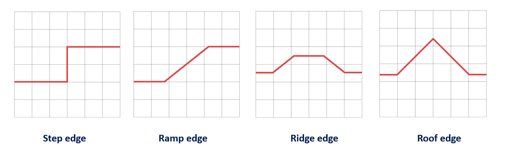
在边缘检测过程中，梯度幅值对噪声极其敏感。Canny检测中，边被定义为像素强度的不连续，或者更简单地说，像素值的急剧差异和变化。

几种边缘示例

Canny边缘检测步骤

噪声去除：使用[[Opencv高级处理#高斯模糊 cv2.GaussianBlur|高斯模糊]]等去除图片噪声，做平滑处理
计算图像梯度：对平滑后的图像使用[[Opencv高级处理#Sobel and Scharr kernels|Sobel算子]]计算水平方向和竖直方向的一阶导数(Gx 和Gy)。根据得到的这两幅梯度，找到边界梯度和方向
非极大值抑制（ Non-maxima suppression）：在获得梯度的方向和大小之后，对整幅图像进行扫描（通常是3×3），去除那些非边界上的点。对每一个像素进行检查，看这个点的梯度是不是周围具有相同梯度方向的点中最大的（如果中心像素的大小大于与之比较的两个像素，则保留，否则丢弃）
滞后阈值（ Hysteresis thresholding）：确定真正的边界，设置两个阈值: TminVal 和TmaxVal。当图像的灰度梯度高于TmaxVal时被认为是真的边界，低于TminVal的边界会被抛弃

调用方法，需要设定上下界的阈值

image = cv2.Canny(blurred, TminVal, TmaxVal)

自动canny代码

实际上这个auto_canny代码已经集成在了imutils中，可以直接调用

import argparse  
import cv2  
import numpy as np  
  
def auto_canny(image, sigma=0.33):  
    v = np.median(image)  
    # apply automatic Canny edge detection using the computed median  
    lower = int(max(0, (1.0 - sigma) * v))  
    upper = int(min(255, (1.0 + sigma) * v))  
    edged = cv2.Canny(image, lower, upper)  
    return edged  
  
ap = argparse.ArgumentParser()  
ap.add_argument("-i", "--image", required=True, help="Path to the image")  
args = vars(ap.parse_args())  
  
image = cv2.imread(args["image"])  
gray = cv2.cvtColor(image, cv2.COLOR_BGR2GRAY)  
blurred = cv2.GaussianBlur(gray, (3, 3), 0)  
  
wide = cv2.Canny(blurred, 10, 200)  
tight = cv2.Canny(blurred, 225, 250)  
auto = auto_canny(blurred)  
  
cv2.imshow("Original", image)  
cv2.imshow("Wide", wide)  
cv2.imshow("Tight", tight)  
cv2.imshow("Auto", auto)  
cv2.waitKey(0)

参考 OpenCV Edge Detection ( cv2.Canny )

轮廓近似

OpenCV Contour Approximation，称为Ramer–Douglas–Peucker 算法
目的是通过减少给定阈值的折线顶点来简化折线。通俗地说，我们取一条曲线，减少它的顶点数量，同时保留它的大部分形状

主要使用cv2.findContours函数寻找所有的轮廓，再使用cv2.approxPolyDP对轮廓进行近似。

import numpy as np  
import argparse  
import imutils  
import cv2  
# construct the argument parser and parse the arguments  
ap = argparse.ArgumentParser()  
ap.add_argument("-i", "--image", type=str, default="shape.png",  
   help="path to input image")  
args = vars(ap.parse_args())  
  
# load the image and display it  
image = cv2.imread(args["image"])  
cv2.imshow("Image", image)  
  
# convert the image to grayscale and threshold it  
gray = cv2.cvtColor(image, cv2.COLOR_BGR2GRAY)  
thresh = cv2.threshold(gray, 200, 255,  
   cv2.THRESH_BINARY_INV)[1]  
cv2.imshow("Thresh", thresh)  
  
# find the largest contour in the threshold image  
cnts = cv2.findContours(thresh.copy(), cv2.RETR_EXTERNAL,  
   cv2.CHAIN_APPROX_SIMPLE)  
cnts = imutils.grab_contours(cnts)  
c = max(cnts, key=cv2.contourArea)  
  
# draw the shape of the contour on the output image, compute the  
# bounding box, and display the number of points in the contour  
output = image.copy()  
cv2.drawContours(output, [c], -1, (0, 255, 0), 3)  
(x, y, w, h) = cv2.boundingRect(c)  
text = "original, num_pts={}".format(len(c))  
cv2.putText(output, text, (x, y - 15), cv2.FONT_HERSHEY_SIMPLEX,  
   0.9, (0, 255, 0), 2)  
  
# show the original contour image  
print("[INFO] {}".format(text))  
cv2.imshow("Original Contour", output)  
cv2.waitKey(0)  
  
# to demonstrate the impact of contour approximation, let's loop  
# over a number of epsilon sizes  
for eps in np.linspace(0.001, 0.05, 10):  
   # approximate the contour  
   peri = cv2.arcLength(c, True) # 计算周长  
   approx = cv2.approxPolyDP(c, eps * peri, True)  
   # draw the approximated contour on the image  
   output = image.copy()  
   cv2.drawContours(output, [approx], -1, (0, 255, 0), 3)  
   text = "eps={:.4f}, num_pts={}".format(eps, len(approx))  
   cv2.putText(output, text, (x, y - 15), cv2.FONT_HERSHEY_SIMPLEX,  
      0.9, (0, 255, 0), 2)  
   # show the approximated contour image  
   print("[INFO] {}".format(text))  
   cv2.imshow("Approximated Contour", output)  
   cv2.waitKey(0)

通过改变eps的值，一步步的近似轮廓边缘。

参考 # OpenCV Contour Approximation

乱谈府

乱谈府